One of the segments of the US economy that was affected most by the Great Recession was consumption. This column use individual-level data to understand the channels through which the decline in house values affected consumption during the Great Recession. The authors find that household-level financial constraints, including those that may have existed previously as well as those triggered by the decline in house values, were responsible for 67% of the decline in consumption. Indirect effects of the decline in house values account for the remaining 33%. The authors find no role for a pure wealth effect.
The Great Recession remains the longest US recession since the Great Depression, and one with long-lasting effects in every part of the economy. One of the segments of the economy that was affected the worst was consumption. There has been considerable work on the empirical front trying to understand why consumption responded so strongly in this period. Mian and Sufi (2009, 2011) and Mian et al. (2013) emphasise the importance of the decline in house prices as a key factor (see also the Vox column here). In their analysis, which uses county-level and ZIP code-level data, they demonstrate that differences in household leverage across these geographic units account for an important part of the consumption decline.
To date, all work that analyses the link between house prices and consumption during the Great Recession has used data that are aggregated to some geographic unit. In a recent paper (Aruoba, Elul and Kalemli-Ozcan, 2022) we use individual-level data to understand the importance of household heterogeneity due to financial constraints, something the existing literature cannot directly capture due to the aggregate nature of the data used. We are also able to unpack these constraints and show that they are composed of financial constraints that may have existed before the Great Recession, as well as those that were triggered by the decline in house values.
House prices and consumption during the Great Recession
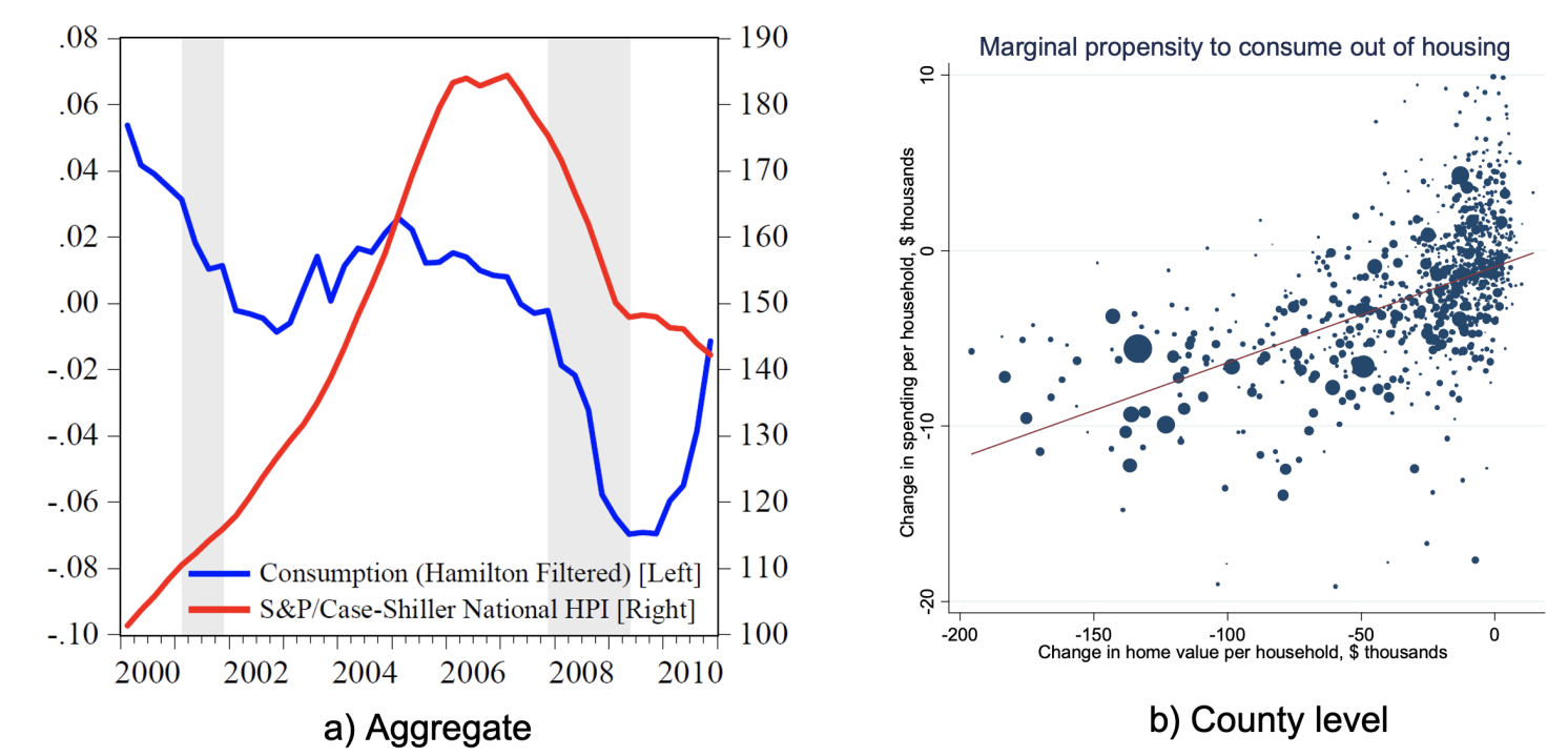
Figure 1 shows the relationship between house prices and consumption in two different ways. Panel (a) shows the relationship between the aggregates over the period 2000-2010. Panel (b), which is taken from Mian et al. (2013), shows the relationship at the county level where the change in consumption between 2006 and 2009 is plotted against the change in home values in the same period. The positive relationship in panel (b) is strong and large: Mian et al.’s ZIP code-level results show a $1,000 drop in house prices leading to a $18 decline in consumption. Using the average house price decline of $47,500, their results suggest a decline of $855 in consumption for the average consumer. Panel (a) shows that while the relationship between the two series has been negative (2000-2002) or non-existent (2002-2006) at times, during the Great Recession (the grey shaded area) it was strongly positive. While these figures show that at the aggregate level there is a strong effect of house price changes on consumption, they cannot address how heterogenous this relationship may be at the household level.
Figure 1 Consumption and house prices


Individual-level data
The biggest obstacle to individual-level analysis of the kind that is needed to answer this question is the availability of individual-level consumption data along with information on individual-level characteristics. We merge two individual-level datasets to this end. One is credit-bureau data from the Federal Reserve Bank of New York Consumer Credit Panel/Equifax (CCP). The other is matched data on residential mortgage originations and performance, along with selected credit bureau variables, from CRISM: Equifax Credit Risk Insight Servicing and Black Knight McDash. In the merged dataset, we have about 349,000 unique individuals with a mortgage at the end of 2006, for whom we are also able to observe balances and delinquency status on a variety of consumer credit obligations, Equifax Risk Scores, as well as detailed information on the mortgages held by the consumer, such as the appraised value of the property and mortgage type. Crucially, our data allow us to compute the dollar change in the consumer’s house value by applying ZIP code-level house price index changes to the appraised value.
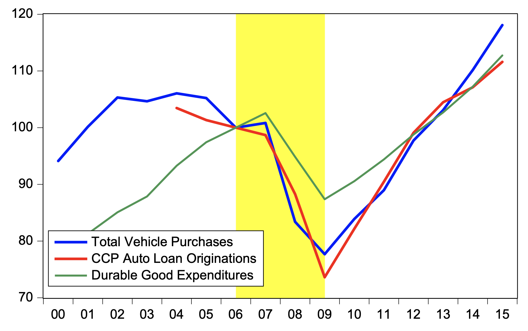
Figure 2 Various aggregate measures of consumption expenditures


We proxy consumption – more specifically, durable consumption – by a binary variable at the individual level that represents if the individual originated an auto loan (including leases) at any point in 2009. Figure 2 shows the aggregate value of this binary variable against ‘Total Vehicle Purchases’ and ‘Durable Good Expenditures’, both produced by the Bureau of Economic Analysis. Our measure tracks the former very well and it seems to be a good proxy for overall durable consumption as well.
Decomposing the link between house values and consumption
We think about house values having both a direct as well as an indirect effect on consumption. The direct effect comes from two distinct channels: the pure wealth effect, and the effect of household-level financial constraints that are influenced by the change in house values. The former effect captures any change in consumption that is unrelated to changes in constraints but simply because the household is now more or less wealthy. The latter is triggered when household-level credit constraints become more (or less) binding as a result of a change in house values. For example, an increase in house values may reduce the loan-to-value (LTV) ratio of the consumer’s mortgage and allow them to refinance at a lower interest rate, or allow them to use a home equity line of credit to extract some of this increased value.
Indirect effects come from channels that do not directly affect a household’s consumption decision but affect some other factors, which ultimately affect consumption decisions. We have two sources of indirect effects in mind: local general equilibrium feedback and bank health. The former channel captures how an initial decline in consumption due to the direct effect of decline in house values feeds back into the economy and makes consumption decline further. (For example, the initial decline in consumption can lead to local firms laying off some workers and then to a further decline in consumption due to the reduced demand by these workers.) The latter channel picks up the effect of the decline in house prices on the asset value of mortgages that banks hold and how this decline translates to a decline in the ability of banks to make further loans. To capture these two channels, we introduce two county-level controls: the change in the unemployment rate between 2006 and 2009, and a credit supply proxy computed along the lines of Gilchrist et al. (2017) and Greenstone et al. (2020).
Our main result involves the effect of changes in house values between 2006 and 2009 on the probability of originating an auto loan in 2009, expressed as a marginal effect computed at the means in dollar terms for ease of comparison. The total effect of the change in house values is estimated to be $1,193. 2 Once both county-level controls are included, the effect of house value changes goes down by a third to $804. We consider the remaining two thirds to be the direct effect of the change in house values on consumption, and turn next to further understand its origins.
Direct effect of change in house values on consumption
To identify the sources of the direct effect, we proceed in three steps. First, we show that a particular constraint is very important in shaping the consumption response of households. Second, we show how certain characteristics of the household, which we argue are linked to constraints they face, influence the consumption response. Finally, we turn to the importance of the pure wealth effect.
We can group constraints into two broad categories. Ex-post constraints are those that get triggered by the change in house values for the individual. To this end, we construct a measure that we label ‘bad mortgage’, which captures whether the individual has been at least 90 days behind in paying any mortgage or experienced a foreclosure at any point in 2007-2009. We show the following results. The average decline in house values between 2006 and 2009 leads to a 5.8 percentage point increase in bad mortgage – in our data, 7.6% of the consumers experience a bad mortgage event. Having a bad mortgage, in turn, leads to a significant decline in the Equifax Risk Score – the probability of having an Equifax Risk Score below 600 goes up by 56.6 percentage points in the event of a bad mortgage. This, in turn, means that the consumer has reduced access to credit and thus is more likely to have lower consumption in 2009. In fact, we find that having a bad mortgage leads to a 8.5 percentage point decline in the probability of originating an auto loan in 2009. Moreover, the $804 we computed for the direct effect of house value changes on consumption is reduced to $301 once we control for bad mortgage, indicating that a large fraction of this direct effect was in fact due to this particular ex-post constraint.
The second type of constraints we consider are ex-ante constraints which predate the decline in house values and are responsible for the housing and borrowing choices the consumers made prior to 2006 and shape their characteristics. Some of the characteristics we consider are the LTV, ex-ante credit worthiness and type of mortgage held – all measured in 2006. We find that consumers with high credit-worthiness (defined as having an Equifax Risk Score of 700 or more) do not respond to changes in house values. Of the other consumers, LTV is an important determinant for the consumption response, with high-LTV consumers responding at least twice as much as the average. Finally, having a closed-end second mortgage (a junior lien that is typically used when the borrower cannot provide a 20% downpayment) also makes a big difference: consumers with lower credit-worthiness, high LTV and a closed-end second mortgage have a consumption response to house value changes over 11 times the average response. This group accounts for about 60% of the overall response despite making up only 4% of all consumers. This result demonstrates both the heterogeneity across consumers as well as the relevance of the ex-ante constraints in shaping consumption decisions in future periods when they interact with changes in house values.
Lastly, we find the pure wealth effect to be negligible. We do this by studying two types of consumers that are unlikely to be financially constrained in response to house price movements, so that any consumption response would be solely due to a wealth effect. First, we focus on consumers with high credit worthiness and very low LTV – so low that even a massive decline in house values does not make them ‘under water’ (i.e. having a level of debt that exceeds the value of their house). With such low LTVs, we consider these households as having no financial constraints that can bind due to a decline in house values. We also consider ‘free and clear’ homeowners without a mortgage. For both types of homeowners, we find that their consumption does not respond to changes in their house values.
To conclude, our results suggest that household-level financial constraints have been very influential in their effect on consumer behaviour once house values started to go down in 2007-2009, and that the impact of these constraints is very heterogeneous. We estimate that they explain about 67% of the decline in consumption in 2009 that resulted from the decline in house values. The remaining 33% can be explained by a combination of local general equilibrium feedback and the impact of house price declines on bank health.
Source : VOXEu


